London School of Economics and Political Science
Outline
Evolutionary stable strategies (ESS)
Basic concepts
Basic concepts I
Intuitively, an evolutionarily stable strategy (ESS) has the property that, if everyone follows it, no other strategy can invade.
To see why a Nash equilibrium does not suffice for evolutionary stability, consider the following game:
| $A$ | $B$ | |
| $A$ | 2, 2 | 1, 1 |
| $B$ | 1, 1 | 1, 1 |
The Nash equilibrium solution concept allows for evolutionary drift.
Basic concepts II
Let $s$ and $s^*$ be two different strategies (behaviours, phenotypes) available to members of the population. In addition, let
- $p$ denote the frequency of $s$ in the population, so the frequency of $s^*$ is $1-p$.
- $W(s)$ and $W(s^*)$ denote the expected fitness of individuals following $s$ and $s^*$, respectively.
- $\pi(s\mid s^*)$ denote the payoff to an individual following strategy $s$ against strategy $s^*$ (with similar meanings for other strategy pairings).
Basic concepts III
If each individual engages in one interaction, and pairings between individuals are at random, then the respective fitnesses of individuals following $s$ and $s^*$ are: $$ W(s) = \underbrace{W_0}_{\text{base fitness}} + \underbrace{p \cdot \pi(s | s) + (1-p)\cdot \pi(s| s^*)}_{\text{expected fitness payoff from a single interaction}} $$ and $$ W(s^*) = \underbrace{W_0}_{\text{base fitness}} + \underbrace{p \cdot \pi(s^* | s) + (1-p)\cdot \pi(s^*| s^*)}_{\text{expected fitness payoff from a single interaction}} $$
Basic concepts IV
If $s^*$ is evolutionarily stable, then $W(s^*) > W(s)$. Therefore,
- If $p\ll 1$, we can ignore terms containing $p$. So $W(s^*) > W(s)$ implies $\pi(s^*| s^*) > \pi(s| s^*)$.
- If, however, $p$ is larger and $\pi(s^*| s^*) = \pi(s| s^*)$, we need to consider the terms containing $p$. In this case, $W(s^*) \gt W(s)$ requires that $\pi(s^* | s) \gt \pi(s|s)$.
Evolutionarily stable strategies I
Putting all these ideas together, we arrive at the following.
- either $\pi(s^*| s^*) > \pi(s|s^*)$
- or $\pi(s^*| s^*) = \pi(s|s^*)$ and $\pi(s^*| s) \gt \pi(s|s)$.
Evolutionarily stable strategies II
There are two logically equivalent ways of writing the definition:
A strategy $s^*$ is evolutionarily stable iff for all strategies $s\neq s^*$
- either $\pi(s^*| s^*) > \pi(s|s^*)$
- or $\pi(s^*| s^*) = \pi(s|s^*)$ and $\pi(s^*| s) \gt \pi(s|s)$.
- $\pi(s^*|s^*) \geq \pi(s|s^*)$
- If $\pi(s^*|s^*) = \pi(s|s^*)$ then $\pi(s^*|s) > \pi(s|s)$
- either $\pi(s^*| s^*) > \pi(s|s^*)$
- or $\pi(s^*| s^*) = \pi(s|s^*)$ and $\pi(s^*| s) \gt \pi(s|s)$.
An alternative definition of an ESS
The first definition given was by Maynard Smith and Price (1973). Another common definition, provably equivalent to it, is as follows.
Some examples
| C | D | |
| C | 2, 2 | 0, 3 |
| D | 3, 0 | 1, 1 |
D is the unique best reply to any mixed strategy, so D is the only ESS.
| $S_1$ | $S_2$ | |
| $S_1$ | 2, 2 | 0, 0 |
| $S_2$ | 0, 0 | 1, 1 |
Both $S_1$ and $S_2$ are the unique best reply to themselves, so each is an ESS, even though one is collectively suboptimal.
Symmetric games
So far, it has been implicit in the discussion that we are only speaking of two-player symmetric games: ones where the assignment of players to Row or Column does not matter. For example:
| S_1 | S_2 | |
| S_1 | a,a | b,c |
| S_2 | c,b | d,d |
The notation $\pi(x|y)$ presupposes symmetric games.
Properties of an ESS
Some games have no ESS I
Consider the game of Rock-Scissors-Paper:
| R | S | P | |
| R | 0, 0 | 1, -1 | -1, 1 |
| S | -1, 1 | 0, 0 | 1, -1 |
| P | 1, -1 | -1, 1 | 0, 0 |
- This game has no Nash equilibrium in pure strategies, so it has no ESS in pure strategies.
- It has one mixed strategy Nash equilibrium, $\sigma = \tuple{\frac13, \frac13, \frac13}$.
Some games have no ESS I
Consider the game of Rock-Scissors-Paper:
| R | S | P | |
| R | 0, 0 | 1, -1 | -1, 1 |
| S | -1, 1 | 0, 0 | 1, -1 |
| P | 1, -1 | -1, 1 | 0, 0 |
Now, $\pi(\sigma|\sigma) = \frac13 \pi(R|\sigma) + \frac13 \pi(S|\sigma) + \frac13\pi(P|\sigma) = 0$.
But $\pi(R | \sigma) = 0$, so we need to check the other condition (from definition 1).
Since $\pi(\sigma|R) = 0$ and $\pi(R|R)=0$, this game has no ESS.
ESS and weakly dominated strategies
Proof: Suppose $\sigma$ is a Nash equilibrium strategy weakly dominated by $\mu$. That is, for all strategies $\tau$, it is the case that $\pi(\mu|\tau) \geq \pi(\sigma|\tau)$ and there exists at least one strategy $\tau^*$ such that $\pi(\mu|\tau^*) > \pi(\sigma|\tau^*)$.
Since $\sigma$ is a Nash equilibrium, it must be the case that $\pi(\mu|\sigma) = \pi(\sigma|\sigma)$. But then, when we check the second condition in the Maynard Smith definition of an ESS, we find that it fails: the fact that $\mu$ weakly dominates $\sigma$ means that $\pi(\mu|\mu) \geq \pi(\sigma|\mu)$.
The support of an ESS
- If $\mu$ is a strategy and $\supp(\mu) \subset \supp(\sigma)$, then $\mu$ is not an ESS.
- If $\mu$ is an ESS with $\supp(\mu) = \supp(\sigma)$, then $\mu=\sigma$.
Proof: Suppose that $\sigma$ is an ESS. We will first show that the expected payoff of any two pure strategies in the support of $\sigma$ are equal, when played against $\sigma$.
The support of an ESS
Proof, continued
To see why, suppose that, to the contrary, there are $x,y\in \supp(\sigma)$ such that $\pi(x|\sigma) > \pi(y|\sigma)$.
For each pure strategy $s\in \supp(\sigma)$, let $p_s$ denote the probability assigned to $s$ by $\sigma$. In particular, $p_x$ and $p_y$ are the probabilities assigned to $x$ and $y$, respectively.
Now consider the strategy $\sigma'$ which plays $x$ with probability $p_x+p_y$, plays $y$ with probability 0, and plays all other pure strategies $s\in \supp(\sigma)$ with probability $p_s$.
The support of an ESS
Proof, continued
Then $$ \pi(\sigma|\sigma) = p_x\pi(x|\sigma) + p_y\pi(y|\sigma) + \sum_{\begin{subarray}{c} s\in \supp(\sigma)\\s\neq x,y\end{subarray}} p_s\pi(s|\sigma) $$
and $$ \pi(\sigma'|\sigma) = (p_x+p_y)\pi(x|\sigma) + 0\cdot\pi(y|\sigma) + \sum_{\begin{subarray}{c} s\in \supp(\sigma)\\s\neq x,y\end{subarray}} p_s\pi(s|\sigma). $$
That means $\pi(\sigma' | \sigma) > \pi(\sigma| \sigma)$, since $\pi(x|\sigma) > \pi(y|\sigma)$. However, that contradicts the assumption that $\sigma$ is an ESS. Hence $\pi(x| \sigma) = \pi(y | \sigma)$ for all $x,y \in \supp(\sigma)$.
The support of an ESS
Proof, continued
Let $\mu$ be a strategy such that $\supp(\mu) \subset \supp(\sigma)$, where $\mu = \sum_{s\in\supp(\mu)} q_s s$. Then $$ \pi(\sigma| \sigma) = \sum_{s\in \supp(\sigma)} p_s \pi(s| \sigma) = \sum_{s \in \supp(\mu)} q_s \pi(s| \sigma) = \pi(\mu | \sigma) $$ as the two middle quantities are merely different convex combinations of equal quantities. Since $\sigma$ is an ESS, the second clause of the Maynard Smith definition requires that $\pi(\sigma | \mu) > \pi(\mu | \mu)$, and so $\mu$ is not an ESS.
Finally, suppose $\mu$ is an ESS with $\supp(\mu) = \supp(\sigma)$, but $\mu\neq \sigma$. This yields a contradition with $\mu$ being ESS (via the above equation), and so $\mu = \sigma$.
Some further consequences
There are some trivial consequences of the last theorem.
Finding an ESS
Finding an ESS
How does one calculate an ESS for a game, if it has one?
- Use the Fundamental Theorem of Mixed Strategy Nash Equilibrium to find a Nash equilibrium.
- Then verify that the Nash equilibrium satisfies the definition of an ESS.
Example: The Hawk-Dove game
In the Hawk-Dove game, two individuals compete for a resource whose possession increases individual fitness. There are two strategies available to each opponent:
- Hawk
- Escalate and continue escalating until opponent retreats or until personal injury occurs.
- Dove
- Display, retreating immediately if opponent escalates.
Denote the fitness value of the resource by $V$ and the fitness cost incurred when personal injury occurs by $C$.
Suppose that, if two Hawks meet, each is equally likely to be injured, and that, if two Doves meet, they share the resource.
Example: The Hawk-Dove game
| Hawk | Dove | |
| Hawk | \frac{V-C}2, \frac{V-C}2 | V, 0 |
| Dove | 0, V | \frac V2, \frac V2 |
Recall the definition of an ESS.
- D is not an ESS because $\pi(D|D) = {V\over 2}$ and $\pi(H|D)=V$, which means that $\pi(D|D)<\pi(H|D)$.
- H is an ESS if $V>C$ because, then, $\pi(H|H)={V-C\over 2}>0$ and $\pi(D|H)=0$, so $\pi(H|H)>\pi(D|H)$.
Example: The Hawk-Dove game
What if $V \lt C$? Neither H nor D is an ESS in this case.
Two questions:
- What happens if individuals can adopt mixed strategies? (That is, acting as a Hawk with probability $p$ and acting as a Dove with probability $1-p$.)
- What happens in a mixed population containing both Hawks and Doves?
Two answers:
- If individuals can adopt mixed strategies, we can use the Fundamental Theorem of Nash Equilibrium to find the ESS.
- In a population containing both Hawks and Doves, there may be a stable polymorphism. (That is, the population proportions won't change under selection pressure.)
Example: The Hawk-Dove game
Applying the Bishop-Cannings theorem
| Hawk | Dove | |
| Hawk | \frac{V-C}2, \frac{V-C}2 | V, 0 |
| Dove | 0, V | \frac V2, \frac V2 |
Straightforward calculations give: \begin{align*} \pi(H|s^*) &= \pi(D|s^*)\\ p\pi(H|H) + (1-p) \pi(H|D) &= p\pi(D|H) + (1-p)\pi(D|D) \\ p\left( \tfrac{V-C}{2}\right) + (1-p)V &= p\cdot 0 + (1-p)\tfrac{V}{2} \\ p &= \tfrac{V}{C} \end{align*}
Since $0 \lt V \lt C$, it follows that $0 \lt p \lt 1$. Moreover, as $V\to C$, $p$ converges to $1$, and we know H is the ESS when $V>C$.
Example: The Hawk-Dove game
Applying the Bishop-Cannings theorem
We have shown that $s^* = pH + (1-p)D$, where $p={V\over C}$, is a Nash equilibrium. We still need to verify that it is an ESS.
Consider a mutant following strategy $\mu = qH + (1-q)D$. Since $\pi(H|s^*) = \pi(D|s^*) = \pi(s^*|s^*)$, it follows that \begin{align*} \pi(\mu|s^*) &= q\pi(H|s^*) + (1-q)\pi(D|s^*) \\ &= q\pi(s^*|s^*) + (1-q)\pi(s^*|s^*) \\ &= \Bigl(q + (1-q)\Bigr)\pi(s^*|s^*) \\ &= \pi(s^*|s^*). \end{align*}
We must show the second clause in the definition of an ESS is satisfied. I leave this as an exercise.
Example: The Hawk-Dove game
Applying the Bishop-Cannings theorem
Answer: Since we know that $\pi(\mu|s^*) = \pi(s^*|s^*)$, we need to show $\pi(s^*|\mu) > \pi(\mu|\mu)$. First, straightforward calculation gives us:
\begin{align*} \pi(s^*|\mu) &= pq\cdot \pi(H|H) + p(1-q)\cdot \pi(H|D) + (1-p)(1-q)\cdot \pi(D|D)\\ &= pq\left(\frac{V-C}2\right) + p(1-q)V + (1-p)(1-q)\frac{V}2\\ &= \frac{V(C-2Cq+V)}{2C}, \text{ since $p=\frac VC.$} \end{align*} and \begin{align*} \pi(\mu|\mu) &= q^2\left(\frac{V-C}2\right) + q(1-q)V + (1-q)^2\frac V2\\ &= \frac12 (V-Cq^2). \end{align*}
Example: The Hawk-Dove game
Applying the Bishop-Cannings theorem
We need to show that the following inequality holds: \begin{equation} \tag{1} \frac{V(C-2Cq+v)}{2C}>\frac12 (V-Cq^2). \end{equation}
Well, we can simplify (1) a bit as follows. First, since $0 \lt V \lt C$ we know we can multiply both sides by $2C$ without reversing the inequality. Further algebraic fiddling gives \begin{align*} V(C-2Cq + V) &> C(V-Cq^2)\\ VC - 2VCq + V^2 &> VC - C^2 q^2\\ V^2 - 2VCq + C^2q^2 &> 0\\ (V-Cq)^2 &> 0. \end{align*} If $q\neq \frac{V}{C}$, then the left-hand side is strictly positive.
Example: The Hawk-Dove game
Mixed populations of Hawks and Doves
For a mixed population to be stable, Hawks and Doves must have equal fitness. Suppose that $P$ of the population are Hawks and $1-P$ are Doves. Then \begin{align*} W(H) &= W(D) \\ P\cdot \pi(H|H) + (1-P) \pi(H|D) &= P\cdot \pi(D|H) + (1-P) \pi(D|D). \end{align*}
Notice that this is formally identical to the equation we solved in answering question 1: \begin{align*} \pi(H|s^*) &= \pi(D|s^*)\\ p \pi(H|H) + (1-p) \pi(H|D) &= p \pi(D|H) + (1-p)\pi(D|D) \end{align*}
When there are only two strategies, the proportions at which a polymorphism is evolutionarily stable equals the probabilities used in the evolutionarily stable mixed strategy, and vice-versa. (Not true, in general.)
Summary, so far
- The concept of an ESS provides a static analysis highlighting the role played by mutations.
- The ESS concept is strictly stronger than that of a Nash equilibrium.
- Some games have no ESS.
- We have discussed one means of searching for an ESS.
- However, the Maynard Smith-Price concept of an ESS is not a dynamic concept. We want a dynamic stability concept which maps on to a notion of evolutionary stability.
It is for this reason that we now turn to the replicator dynamics.
The replicator dynamics
Definition
The replicator dynamics
- Let $s_i$ denote the frequency of strategy $i$ in the population, with $\svec = (s_1,\dots,s_n)$.
- Let $W_i$ denote the current fitness of strategy $i$ in the population: \[ W_i = \sum_{j=1}^n s_j\cdot \pi(i | j). \]
- Let $\bar W$ denote the average fitness of the population: \[ \bar W = \sum_{i=1}^n s_i\cdot W_i. \]
The replicator dynamics
The rate of change of strategy $i$ is given by the following system of differential equations: $$ \dot s_i = s_i \Bigl( W_i - \bar W\Bigr). $$
As a model of biological evolution
The replicator dynamics (biological model)
We can interpret the mathematics of the replicator dynamics as describing how changes in phenotype frequencies evolve.
As we will see, this involves a number of important assumptions on how the population interacts and how reproduction occurs.
These specific assumptions are not strictly necessary, for there are other ways of deriving the replicator dynamics — but they are perhaps the most straightforward.
The replicator dynamics (biological model), I
Suppose that:
- Payoffs represent changes in individual fitness, measured in terms of the number of offspring.
- Each offspring follows the same strategy as her parent (i.e., that “strategies breed true”).
- The only thing that matters about individuals is what strategy they follow.
- The population is extremely large (i.e., effectively infinite) and panmictic (i.e., all pairwise interactions between individuals are equally likely — so no population or group structure exists).
The replicator dynamics (biological model), II
- Let $1,\dots,m$ denote phenotypes (strategies) available to members of the population.
- $n_i =$ the number of agents in the population with phenotype $i$.
- $N = \displaystyle\sum_{i=1}^m n_i$ is the total size of the population.
- Given that only the strategy adopted by an individual matters, along with the assumption of panmicticity, all of the relevant information about the population is contained in the state vector \[ \svec=(s_1,\dots,s_m) \] where $s_i=\frac{n_i}{N}$.
The replicator dynamics (biological model), III
- If reproduction takes place continuously, the average birth rate for individuals of type $i$ is $$ \underbrace{W_0}_{\text{background fitness}} + \underbrace{W_i}_{\text{expected fitness of $i$ in population}} $$ where $$ W_i = \sum_{j=1}^m s_j\cdot \pi(i|j). $$
- If $\delta$ denotes the common death rate, the rate of change in the number of individuals with phenotype $i$ is \[ \dot n_i = \Bigl( W_0 + W_i - \delta \Bigr) n_i. \]
The replicator dynamics (biological model), IV
The rate of change of the population frequencies is easily shown to be \[ \dot s_i = \Bigl( W_i - \bar W\Bigr) s_i. \]
(How? Recall that $s_iN=n_i$. Take the time derivative of both sides and simplify.)
And thus we arrive at the replicator dynamics, introduced by Taylor and Jonker (1978).
Some examples
Some examples
The Prisoner's Dilemma
| C | D | |
| C | 2, 2 | 0, 3 |
| D | 3, 0 | 1, 1 |
Some examples
The Driving game (a coordination problem)
| L | R | |
| L | 1, 1 | 0, 0 |
| R | 0, 0 | 1, 1 |
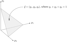
Representing a three-dimensional state space
Some examples
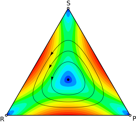
Rock-Scissors-Paper
| R | S | P | |
| R | 1, 1 | 2, 0 | 0, 2 |
| S | 0, 2 | 1, 1 | 2, 0 |
| P | 2, 0 | 0, 2 | 1, 1 |
Some examples
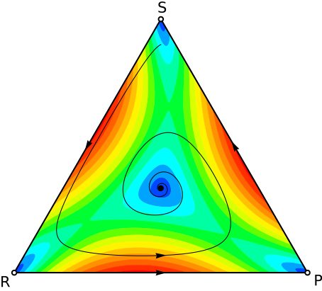
“Good” Rock-Scissors-Paper
| R | S | P | |
| R | 1, 1 | 2.5, 0 | 0, 2.5 |
| S | 0, 2.5 | 1, 1 | 2.5, 0 |
| P | 2.5, 0 | 0, 2.5 | 1, 1 |
Some examples
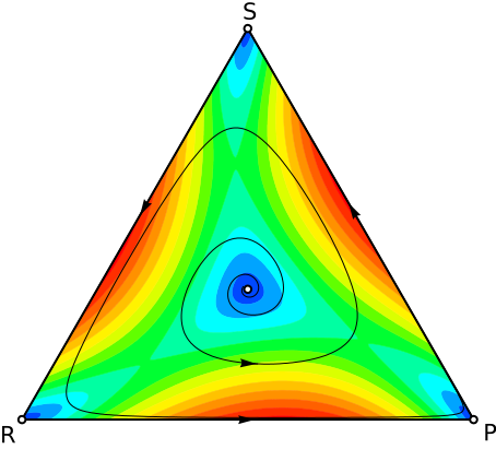
“Bad” Rock-Scissors-Paper
| R | S | P | |
| R | 1, 1 | 1.5, 0 | 0, 1.5 |
| S | 0, 1.5 | 1, 1 | 1.5, 0 |
| P | 1.5, 0 | 0, 1.5 | 1, 1 |
Interactive replicator dynamics
A brief discussion about stability
Different stability concepts
Two classic notions of stability which are relevant for the replicator dynamics are Lyapunov stability and asymptotic stability. Since we only need the intuitive idea, I won't present formal definitions.
Asymptotic stability $\neq$ being a global attractor
- In Skyrms's Evolution of the Social Contract, much is made of the fact that certain states are attractors (sometimes global attractors) of the replicator dynamics.
- Be careful not to confuse these two concepts. A state can be a global attractor while not being asymptotically stable (Ritzberger and Weibull, 1995):
| A | B | C | |
| A | 0, 0 | 1, 0 | 0, 0 |
| B | 0, 1 | 0, 0 | 2, 0 |
| C | 0, 0 | 0, 2 | 1, 1 |
Asympotically stable states and ESS
One can prove [see Weibull, 1995; Taylor and Jonker, 1978; and Hofbauer et al., 1979] that, for the continuous-time replicator dynamics, a very close relationship exists between ESS and asymptotically stable states:
Some caveats:
- This need not hold for the discrete-time replicator dynamics.
- Why? If time is too coarsely grained, the discrete replicator dynamics can “jump past” the asymptotically stable state.
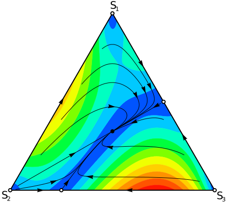
An asymptotically stable state may not be ESS
Note that the converse of the previous theorem does not hold.
| $S_1$ | $S_2$ | $S_3$ | |
| $S_1$ | 1, 1 | 1, 0 | 1, 0 |
| $S_2$ | 0, 1 | 0, 0 | 3, 1 |
| $S_3$ | 2, 1 | 1, 3 | 0, 0 |
An ESS can have an arbitrarily small basin of attraction
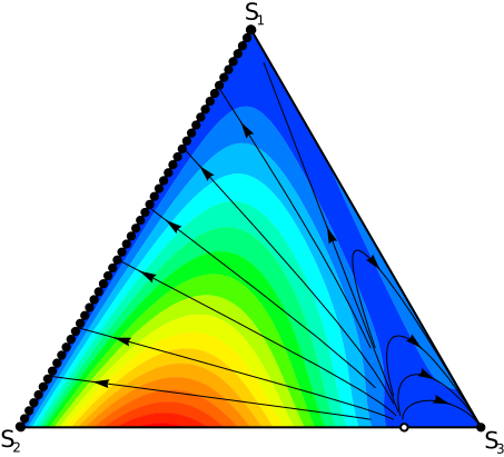
This game shows that an ESS may not be explanatorily significant.
| S_1 | S_2 | S_3 | |
| S_1 | 0, 0 | 1, 0 | \epsilon, 0 |
| S_2 | 0, 1 | 1, 1 | 0, 0 |
| S_3 | 0, \epsilon | 0, 0 | 2\epsilon, 2\epsilon |
Bounded rationality and strictly dominated strategies
Learning rules and population behaviour
In Population Games and Evolutionary Dynamics, William Sandholm offers a useful framework for thinking about the connection between an individual’s learning rules and the aggregate dynamics of the population.
The key idea is the conditional switch rate \(\rho_{ij}\), the rate at which an agent currently playing strategy \(S_i\) switches to strategy \(S_j\).
Different forms of \(\rho_{ij}\) represent different assumptions about what agents know and how they revise their behaviour.
This yields differences at the population level.
The Replicator Dynamic
Belief-revision process: Imitative learning.
An agent playing \(S_i\) samples another agent at random. If that agent plays \(S_j\) and does better than average, switch with probability proportional to the payoff difference: \[ \rho_{ij} \;=\; p_j \,\bigl[W_j - \bar{W}\bigr]_+ \]
This yields the replicator equation: \[ \dot{p}_i \;=\; p_i\!\left(W_i - \bar{W}\right) \]
Note the factor \(p_j\): you can only imitate strategies already present in the population.
The limits of imitation
Two consequences of the replicator’s reliance on \(p_j\):
-
No Innovation. If \(p_j = 0\), then \(\rho_{ij} = 0\).
Strategies absent from the population can never be introduced.
-
Fails Nash Stationarity.
Every vertex of the simplex is a rest point, even vertices
which do not correspond to Nash Equilibria of the underlying game.
E.g., All-Cooperate in the Prisoner’s Dilemma is a fixed point, though unstable.
However, the replicator dynamic always eliminates strictly dominated strategies.
The Brown–Nash–von Neumann Dynamic
Belief-revision process: The rate at which an agent switches to \(S_j\) depends only on whether \(S_j\)’s expected fitness exceeds the population average, independent of the agent’s current strategy or payoff: \[ \rho_{ij} \;=\; \bigl[W_j - \bar{W}\bigr]_+ \]
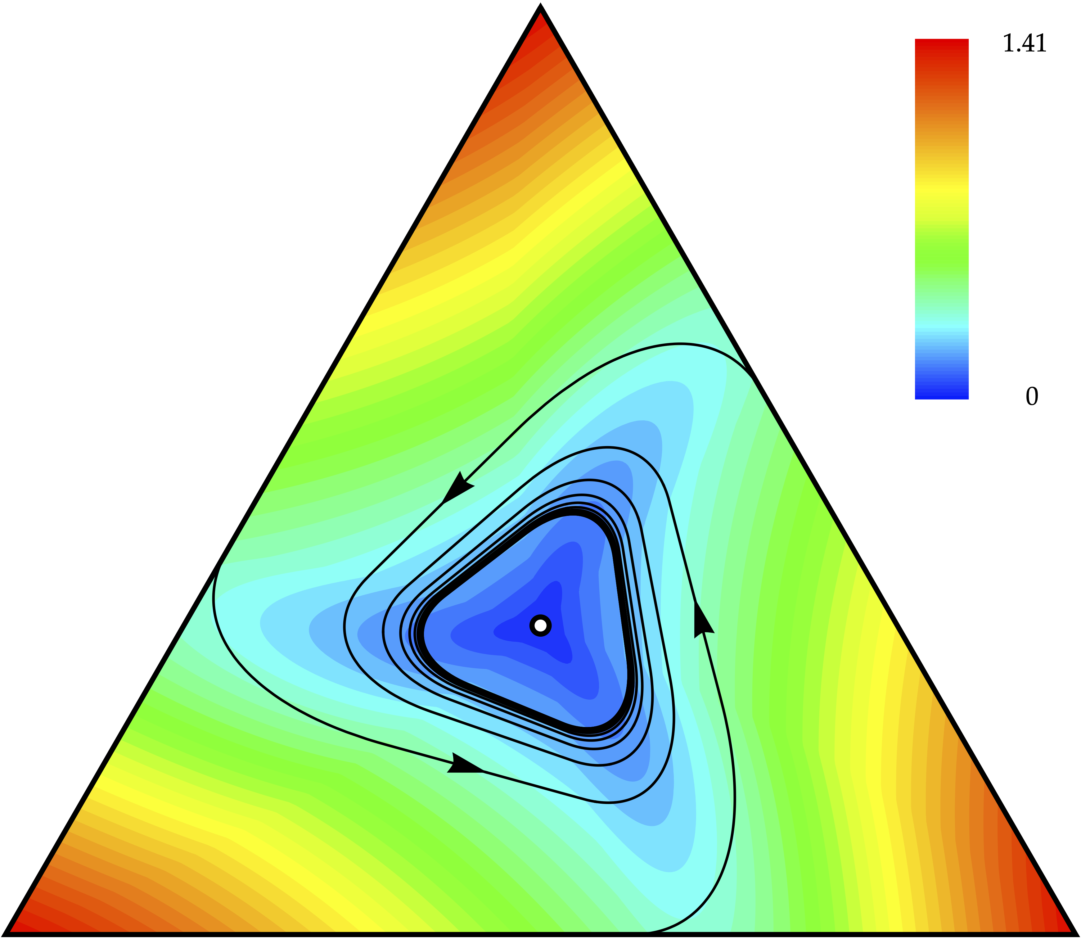
Rational improvement over imitation: the factor \(p_j\) is gone. That means agents can consider strategies not currently represented in the population. But agents remain boundedly rational: any above-average strategy attracts adopters, not just the best response.
BNN in Action: ‘Bad’ Rock-Paper-Scissors
| R | S | P | |
| R | 1, 1 | 1.5, 0 | 0, 1.5 |
| S | 0, 1.5 | 1, 1 | 1.5, 0 |
| P | 1.5, 0 | 0, 1.5 | 1, 1 |
Starting from pure states (all-\(R\), all-\(S\), or all-\(P\)), the BNN dynamic introduces absent strategies into the population.
Under the replicator dynamic, by contrast, a population at a vertex stays there forever.
The Smith Dynamic
Belief-revision process (Smith, 1984): The switch rate from \(S_i\) to \(S_j\) depends on whether \(S_j\)’s expected fitness exceeds that of the agent’s own strategy \(S_i\), rather than the population average: \[ \rho_{ij} \;=\; \bigl[W_j - W_i\bigr]_+ \]
A further rational improvement: This rule avoids distortion introduced by the population average (a poorly performing strategy can drag \(\bar{W}\) down, making mediocre strategies appear attractive under BNN).
Smith’s process bases choices on fitness improvements attainable by actual alternative strategies.
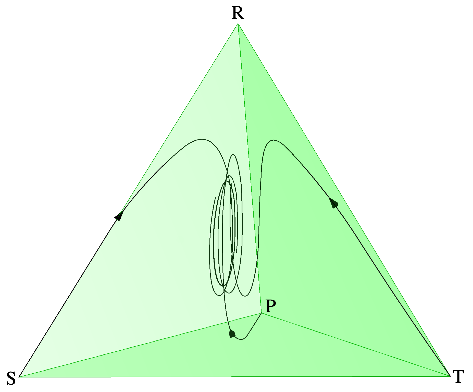
The survival of strictly dominated strategies
Consider bad RPS with a “feeble twin”:
| R | P | S | T | |
| R | (0,0) | (-2,1) | (1,-2) | (1,-2-\epsilon) |
| P | (1,-2) | (0,0) | (-2,1) | (-2,1-\epsilon) |
| S | (-2,1) | (1,-2) | (0,0) | (0,-\epsilon) |
| T | (-2-\epsilon, 1) | (1-\epsilon, -2) | (-\epsilon, 0) | (-\epsilon, -\epsilon) |
The Hofbauer–Sandholm Theorem
Hofbauer & Sandholm (2011) show that preservation of strictly dominated strategies is not peculiar to the Smith dynamic. It follows from four general conditions:
- Continuity. Lipschitz continuity of the growth-rate function.
- Positive Correlation. Strategy growth is positively correlated with payoff.
- Nash Stationarity. Rest points occur only at Nash equilibria.
- Innovation. At a non-Nash population state, optimal strategies have strictly positive growth.
The Hofbauer–Sandholm Theorem
The Paradox
The replicator dynamic eliminates strictly dominated strategies precisely because it is, in some respects, less rational. It models imitative agents who cannot consider strategies absent from the population.
The BNN and Smith dynamics fix this: agents can innovate and only Nash equilibria are stationary. But the capacity for innovation that makes these dynamics more rational sustains dominated strategies.
How so? A strictly dominated “twin” strategy can maintain a positive adoption rate because it still offers fitness improvements over some strategies in the population cycle.
Three dynamics, increasing rationality
| Replicator | BNN | Smith | |
|---|---|---|---|
| \(\rho_{ij}\) | \(p_j[W_j - \bar{W}]_+\) | \([W_j - \bar{W}]_+\) | \([W_j - W_i]_+\) |
| Benchmark | Pop. average | Pop. average | Own strategy |
| Innovation? | ✗ | ✓ | ✓ |
| Nash Stationarity? | ✗ | ✓ | ✓ |
| Eliminates dominated? | Always | Not always | Not always |
Each step makes the individual’s revision process more rational.
Yet the population-level consequence is, paradoxically, less reliable elimination of dominated strategies.
Bibliography
Bibliography
Bishop, D. T. and C. Cannings (1978). “A generalised war of attrition.” Journal of Theoretical Biology, 70: 85–124.
Björnerstedt, Jonas (1993). “Experimentation, imitation, and evolutionary dynamics,” Unpublished working paper. Department of Economics, Stockholm University.
Gigerenzer, Gerd and Peter M. Todd and the ABC Research Group (1999). Simple Heuristics That Make Us Smart. Oxford University Press.
Hofbauer, J.; P. Schuster, and K. Sigmund (1979). “A note on evolutionary stable strategies and game dynamics.” Journal of Theoretical Biology, 81: 609–12.
Maynard Smith, John and George Price (1973). “The Logic of Animal Conflict.” Nature, 246: 15–18.
Ritzberger, K. and J. Weibull (1995). “Evolutionary selection in normal-form games.” Econometrica, 63: 1371–99.
Skyrms, Brian (1996). Evolution of the Social Contract. Cambridge University Press.
Taylor, Peter D. and Leo B. Jonker (1978). “Evolutionary Stable Strategies and Game Dynamics.” Mathematical Biosciences, 40: 145–156.
Weibull, Jörgen W. (1995). Evolutionary Game Theory. The MIT Press.
Appendix
The replicator dynamics (cultural model)
We can interpret the mathematics of the replicator dynamics as describing how changes in the frequency of behaviour evolve, based on learning from experience.
As we will see, this also involves a number of important assumptions on how the population interacts and how learning takes place.
These specific assumptions are not strictly necessary, for there are other ways of deriving the replicator dynamics based on individual learning.
The replicator dynamics (cultural model), I
- Suppose we have a population of boundedly rational agents who repeatedly interact and play the game $G$ with strategies $1,\dots,m$.
-
Suppose each agent wants to maximize their payoff from the
game $G$, and so they will change their strategy from time to time
if they believe that they are not doing sufficiently well.
- More precisely, each agent periodically reviews her strategy. At the end of each review process, she may adopt a new strategy.
- Assume each agent following strategy $i$ reviews her strategy at the rate $r_i$.
- Without worrying about the specific heuristic an agent uses to adopt a new strategy, denote the probability that an individual following strategy $i$ will switch to strategy $j$ by $p_i^j$.
The replicator dynamics (cultural model), II
Also assume:
- The number of times an agent reviews her strategy between time $t$ and $t+\Delta t$ does not affect the number of times that she reviews her strategy during another interval $t'$ and $t'+\Delta t'$.
- The average rate that she reviews her strategy remains constant.
- Each agent must finish reviewing her strategy before beginning to review it another time.
If each individual strategy review and strategy switch is independent of every other review and switch, and the population is sufficiently large, then:
- The proportion of the population following strategy $i$ that chooses to review it is $s_ir_i$.
- The proportion of the population following strategy $i$ that switches to another strategy $j$, after review, is $s_ir_i p_i^j$.
The replicator dynamics (cultural model), III
- The total rate at which people start using $i$ is $\displaystyle \sum_{j\neq i} s_j r_j p_j^i.$
- The total rate at which people stop using $i$ is $\displaystyle \sum_{j\neq i} s_i r_i p_i^j.$
- The overall rate of change for the frequency of strategy $i$ is the difference of these two: \begin{align} \tag{2} \frac{ds_i}{dt} &= \left( \sum_{j\neq i} s_j r_j p_j^i \right) - \left(\sum_{j\neq i} s_i r_i p_i^j \right). \end{align}
- Rearranging (2), and noting that $\sum_j p_i^j=1$, the rate of change of strategy $i$ in the population equals \begin{equation} \tag{3} \frac{ds_i}{dt} = \sum_{j=1,\dots,m} s_j r_jp_j^i - r_i s_i. \end{equation}
The replicator dynamics (cultural model), IV
- Gigerenzer (1999) discusses a particular heuristic called the “take the last” heuristic. According to this heuristic, a boundedly rational individual chooses the last option they’ve encountered. In our model, this means that an individual will adopt the strategy held by the last person they've encountered from the population.
- If people mix randomly, the probability that a person following strategy $i$ will adopt strategy $j$ is just the frequency of strategy $j$ in the population. I.e., \[ p_i^j = s_j. \]
The replicator dynamics (cultural model), V
- Björnerstedt (1993) observed that if the review rate decreases linearly with the individual's payoff (which means that individuals review their strategy less often as their payoff increases), we can derive the replicator dynamics from the above.
- The particular review rate Björnerstedt suggested had the following form: \[ r_i = a - b F(i|\svec) \] where $a,b\in \mathbb{R}$ with $b>0$, and $\frac{a}{b} \geq F(i|\svec)$.
- From this, it follows that \[ \frac{ds_i}{dt} = b\Bigl( F(i|\svec) - F(\svec\,|\svec)\Bigr) s_i. \] (How? Take equation (3), substitute in the appropriate values for $r_i$ and $p_i^j$, then simplify.)
The replicator dynamics (cultural model), VI
\begin{equation} \tag{4} \frac{ds_i}{dt} = b\Bigl( F(i|\svec) - F(\svec\,|\svec)\Bigr) s_i. \end{equation}
Notice that equation (4) is simply a rescaled version of the replicator dynamics. If we rescale time, we get the canonical form of the replicator dynamics. (This is also equivalent to setting the free parameter $b=1$.)
In short, a population of boundedly rational individuals who
- choose to review their strategies with a frequency according to their level of dissatisfaction,
- adopt new strategies using the “take the last” heuristic,
evolves (in the cultural evolutionary sense) according to a rescaled version of the continuous replicator dynamics.